The whole limit in ninety seconds

Executive summary

Norway's exposure limits for respirable silica are low (0.05 mg/m³ for quartz, 1.5 mg/m³ for the amorphous form), and it is tempting to conclude that a dust sensor which reads up to 10 mg/m³ has more range than it will ever need. It does not. The limit is an average over an eight-hour shift, and a shift is not eight hours of steady air. In a smelter or a concrete plant most of the day is close to clean, and a handful of short bursts, at tapping, charging, cleaning or a spill, carry most of the dust a worker breathes. A burst of a minute or two can spend the entire day's allowance on its own.

A sensor that cannot measure above its ceiling does not report an error when the air goes past it. It reports the ceiling. The burst is recorded as smaller than it was, the shift average comes out too low, and the plant gets a clean result for a day that was not clean. This error only ever runs one way: a sensor that saturates never raises a false alarm, only a false all-clear, and it does so on exactly the events monitoring exists to catch. The fifteen-minute short-term check does not rescue the situation, because it is computed from the same clipped data.

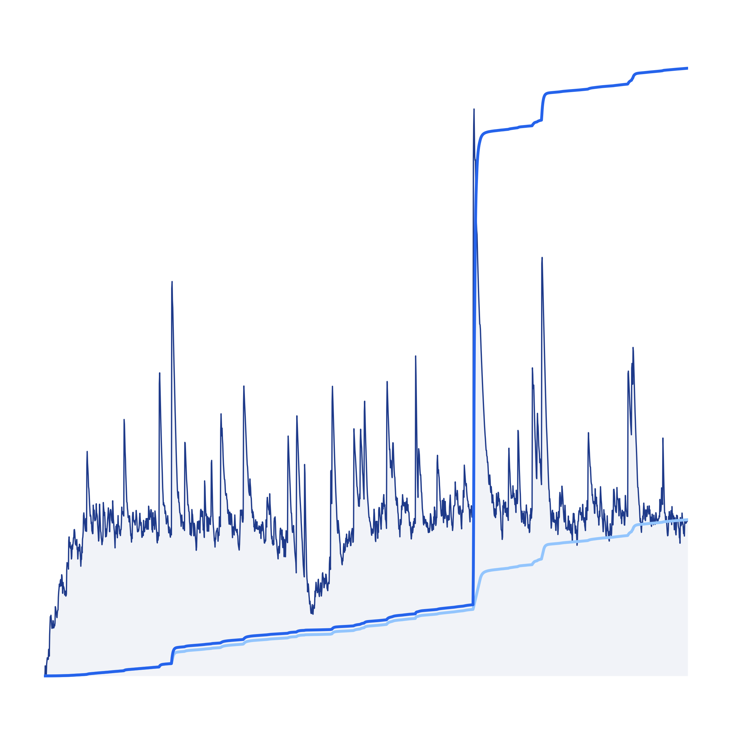
The figure below shows an example of what this looks like: a quiet day around 0.5 mg/m³ with a single tapping plume at 14:20 that peaks near 700 mg/m³ and stays above 10 mg/m³ for five minutes. The true average over eight hours is 2.21 mg/m³, roughly half as much again as the 1.5 mg/m³ limit for amorphous silica. An instrument that stops at 10 mg/m³ reports 0.57 mg/m³, under 40% of the limit, and shows a clean day. Those five minutes carry three quarters of the shift's dose.

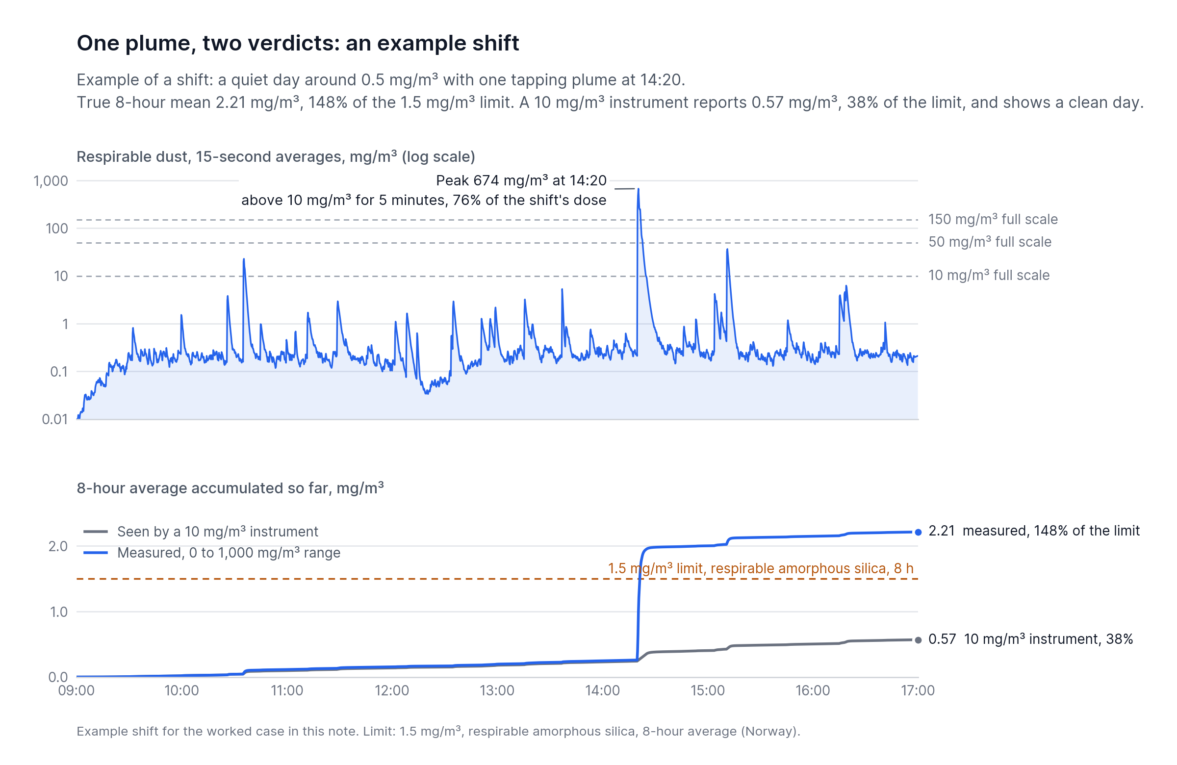
An example shift on a log scale: a quiet day around 0.5 mg/m³ with one tapping plume at 14:20, with three instrument full scales marked. The lower panel shows the eight-hour average building up over the shift, as measured and as an instrument with a 10 mg/m³ ceiling would report it, against the 1.5 mg/m³ limit.

The practical conclusion is that the measurement range of a dust sensor has to be chosen from what the process produces, not from the size of the limit. Ask what the dusty operations reach at the measurement position, and pick an instrument that can follow them. Insist that intervals where the sensor sat at its ceiling are flagged rather than silently averaged in, that the sensor integrates continuously between reports so that short events are never skipped, and that the conversion from scattered light to mass is calibrated on the plant's own dust. A fixed sensor still does not replace personal sampling in a compliance test. What it does is show where and when the exposure happens, so that ventilation and work practice can be aimed at the few minutes that carry the dose.

The rest of this note gives the arithmetic, the worked cases and the specification points behind these conclusions.

1. The limit is an eight-hour average

Norwegian regulation defines the limit value as the maximum permitted mean concentration in a worker's breathing zone over a fixed reference period of eight hours.¹ The corresponding measurement is a filter-based personal sampler: a pump draws air through a cyclone that imposes the respirable size convention of EN 481, and the filter is weighed before and after the shift. The instrument integrates by construction and has no range problem, because mass on a filter does not saturate at any concentration a workplace produces.

Its problem is a different one: it returns one number per shift, weeks later, and that number says nothing about when the exposure happened or what caused it. A plant that fails a gravimetric test learns that it failed, and nothing about what to change.

Real-time optical monitoring exists to fill that gap, and to fill it the instrument has to reproduce the same integral the filter computes:

$${\bar{C}}_{8h}=\frac{1}{T}{\int }_0^{T}C(t)\mathrm{d}tT=8\text{ h}=\mathrm{28,800}\text{ s}$$

Nothing in that expression bounds $C(t)$; the bound is on the average. The instantaneous concentration is set by the process, and in a smelter it climbs into the tens and hundreds of mg/m³ during tapping and charging — one to two orders of magnitude above the amorphous limit, three to four above the quartz limit — for seconds to minutes at a time.

A note on species before the numbers. The limit applies to a chemical species, while an optical sensor measures the respirable fraction of total airborne dust. In silicon and ferrosilicon plants the airborne dust is dominated by microsilica at 85 to 98% amorphous SiO₂, so respirable dust and regulated species are close to interchangeable for the amorphous limit. For the crystalline limit only the quartz fraction counts, and converting one to the other needs the dust composition. None of the dose arithmetic below changes: it applies to whichever species the limit names, at whatever fraction of the measured mass that species represents.

2. The exposure budget

Rewrite the limit as an allowance. If the limit is $L$ and the reference period is $T$, the permitted mass-time product across a shift is

$$D_{\max }=L\cdot T$$

with units of mg·s/m³. For Norway:

Species	Limit $L$	Shift budget $D_{\max }$
Respirable crystalline silica	0.05 mg/m³	1,440 mg·s/m³ = 24 mg·min/m³
Respirable crystalline silica (EU binding value)	0.10 mg/m³	2,880 mg·s/m³ = 48 mg·min/m³
Respirable amorphous silica	1.5 mg/m³	43,200 mg·s/m³ = 720 mg·min/m³

A constant concentration $C$ consumes the whole budget in $t=D_{\max }\mathrm{/}C$. This is the table that decides how much range an instrument needs.

Concentration	Time to spend a full quartz budget (0.05 mg/m³)	Time to spend a full amorphous budget (1.5 mg/m³)
1 mg/m³	24 min	12 h
5 mg/m³	4.8 min	2 h 24 min
10 mg/m³	2.4 min	1 h 12 min
50 mg/m³	28.8 s	14.4 min
100 mg/m³	14.4 s	7.2 min
250 mg/m³	5.8 s	2.9 min
500 mg/m³	2.9 s	1.4 min
1,000 mg/m³	1.4 s	43 s

At the bottom of the table, a worker standing in a 500 mg/m³ plume of quartz-bearing dust exhausts a whole day's allowance in the time it takes to say a sentence.

The same arithmetic answers a second question: when does one event outweigh everything else in the shift? Take a shift at background $B$ containing one excursion of amplitude $A$ and duration $\tau$. The excursion carries more dose than the entire rest of the shift when

$$\tau >\frac{BT}{A+B}$$

At a background of 0.4 mg/m³:

Event amplitude	Duration at which the event outweighs the whole shift
50 mg/m³	3 min 49 s
100 mg/m³	1 min 55 s
300 mg/m³	38 s
600 mg/m³	19 s
1,000 mg/m³	12 s

Nineteen seconds of a tapping plume outweighs seven hours and fifty-nine minutes of ordinary work.

3. What a range ceiling does to the number

Model the instrument as ideal below its full scale $C_{\max }$ and hard-clipped above it:

$$\widehat{C}(t)=\min \text{\hspace{0.17em}⁣}(C(t),C_{\max })$$

The reported average is then

$$\widehat{\bar{C}}=\bar{C}-\frac{1}{T}{\int }_0^T\max \text{\hspace{0.17em}⁣}(C(t)-C_{\max },0)\mathrm{d}t$$

The second term is the dose the instrument cannot see. For a single rectangular excursion of amplitude $A>C_{\max }$ and duration $\tau$ on a background $B$, the reported and true averages are

$$\widehat{\bar{C}}=B+(C_{\max }-B)\frac{\tau }{T},\bar{C}=B+(A-B)\frac{\tau }{T}$$

and when the excursion dominates, the ratio of reported to true dose approaches $C_{\max }\mathrm{/}A$. The error factor is set by how far the peak overshoots full scale, and it does not depend on how good the instrument is inside its range. On this shift, a device with 5% accuracy that clips at 10 mg/m³ stops being a 5% device and becomes a 5× device.

Worked case

Background 0.4 mg/m³. One event: 600 mg/m³ for 90 seconds. Shift 8 h.

True average: 0.399 + 1.875 = 2.274 mg/m³, of which the background contributes 17.5% and the 90-second event contributes 82.5%. The event is 0.31% of shift time.

Full scale	Reported average	Fraction of true	Against $L$ = 1.5 mg/m³	Verdict on screen
10 mg/m³	0.430	18.9%	28.7%	Clear
50 mg/m³	0.555	24.4%	37.0%	Clear
150 mg/m³	0.868	38.2%	57.8%	Clear
300 mg/m³	1.336	58.8%	89.1%	Elevated
1,000 mg/m³	2.274	100%	151.6%	Breach

The figure in the executive summary shows a shift of this kind with a more realistic plume, a fast rise to 674 mg/m³ and a tail that stays above 10 mg/m³ for five minutes. Its averages, 2.21 mg/m³ true and 0.57 mg/m³ on a 10 mg/m³ instrument, land close to the rectangular model's.

Hard clipping is the optimistic model. A real optical particle counter does not stay linear up to a firmware ceiling and then stop. Coincidence-driven compression sets in progressively, well below nominal full scale, and it is usually not flagged in the data stream (section 7 covers the mechanism). So a narrow instrument's true response curve sits below the line drawn above, and its error is larger than this table suggests.

4. The short-term test fails the same way

Brief excursions are supposed to be caught by a separate mechanism. For substances without a specified short-term value (annotation S) or ceiling value (annotation T), Norwegian practice applies an excursion allowance over periods of up to fifteen minutes, expressed as a percentage of the limit:²

Limit value	Permitted excess over 15 minutes
≤ 1	200%
> 1 to 10	100%
> 10 to 100	50%
> 100	25%

The allowance is conditional: it applies only when the eight-hour average is itself within the limit. For amorphous silica at 1.5 mg/m³ it gives a fifteen-minute ceiling of 3.0 mg/m³. Applied to the worked case:

Full scale	Worst 15-min mean	Against the 3.0 mg/m³ ceiling
10 mg/m³	1.36 mg/m³	Passes, at 0.45×
50 mg/m³	5.36 mg/m³	Fails, at 1.8×
150 mg/m³	15.4 mg/m³	Fails, at 5.1×
True	60.4 mg/m³	Fails, at 20×

In the worked case the true eight-hour average is already 152% of the limit, so the allowance does not apply at all. The 10 mg/m³ instrument reports an eight-hour average at 29% of the limit and a worst window at 45% of the ceiling, and passes both tests it should have failed. The test designed to catch short excursions is defeated by an instrument that cannot measure short excursions. The excursion rule looks like the safeguard that makes range irrelevant. It is no safeguard at all against a clipped record, because it is computed from the same clipped record.

5. The failure is asymmetric

Every failure mode discussed so far biases the reading downward. No configuration of range ceiling, coincidence or averaging causes a saturating sensor to overstate a peak.

For a safety instrument this is the wrong direction. Protective instrumentation is normally designed so that faults drive the output toward the alarm state and a failure announces itself. Range saturation does the opposite. It produces plausible, well-behaved data saying the workplace is cleaner than it is, and nothing in the record looks wrong: the trace is smooth, the average is low, the alarms are quiet, and the operator has no signal that anything is missing.

Saturated intervals therefore have to be flagged in the data rather than silently folded into the average. An interval in which the sensor sat at full scale is a measurement of at least full scale, and it should carry through to the reported average as a lower bound with an explicit flag. An average computed across unflagged saturated bins is a censored statistic presented as a complete one.

Range should also be verified rather than assumed. A vendor specification of "0 to X mg/m³" says nothing about behaviour at 1.2X. Ask what the instrument does above full scale: hard clip, progressive roll-off, or an error state. Ask whether the response has been characterised above nominal range or only within it.

6. Cadence: the second way to lose an event

Range decides whether an event is measured correctly; sampling decides whether it is measured at all. Two architectures behave very differently here.

An integrating sensor draws air continuously and reports the true mean over each reporting interval. Dose is preserved exactly, whatever the interval length, provided nothing clips. A 5-second burst at 500 mg/m³ inside a 60-second bin is reported as 41.7 mg/m³: correct in dose, wrong in peak. That is enough for compliance arithmetic but not for alarming and root-cause work, because the reported value never approaches the concentration a worker actually stood in, and correlating it with a discrete process event becomes guesswork.

A snapshot sensor reads instantaneously every $\mathrm{\Delta }t$ and holds the value. An event shorter than $\mathrm{\Delta }t$ is either missed entirely or counted as though it lasted the full interval. The estimator is unbiased in expectation and useless in practice, because its variance is enormous. With catch probability $p=\tau \mathrm{/}\mathrm{\Delta }t$, the coefficient of variation of the single-shift dose estimate is

$$\mathrm{C}\mathrm{V}=\sqrt{\frac{1-p}{p}}=\sqrt{\frac{\mathrm{\Delta }t}{\tau }-1}$$

Event duration	Sampling interval	CV of the dose estimate
5 s	15 s	141%
5 s	60 s	332%
5 s	300 s	768%
30 s	60 s	100%
30 s	300 s	300%

A shift average built from snapshots of a transient process is a lottery ticket. Repeat the same shift five times under identical conditions and you get five wildly different answers, none of them wrong in any way the operator can detect.

So the requirement is continuous integration between reports, with a reporting interval short enough to resolve the events under investigation. Arpuro sensors integrate continuously and report every 15 seconds. A 90-second tapping event spans six reporting intervals, enough to establish its duration and its correlation with a logged operation.

7. Why wide range is hard

Range is fixed by physics. Two constraints pull against each other, and where they meet defines the usable span.

The top end is limited by coincidence. An optical particle counter sizes particles one at a time as they transit an illuminated sensing volume $V$. When two particles occupy $V$ at once, the detector registers one larger particle. Number is undercounted and size is overestimated, and because mass scales as $d^3$ while count scales as $d^0$, the net effect on reported mass is a compressive nonlinearity that grows with concentration. If particle arrivals are Poisson with mean occupancy $\lambda =NV$, the fraction of particles lost to coincidence is

$$f_{\text{lost}}=1-\frac{1-e^{-\lambda }}{\lambda }$$

$\lambda$	Particles lost
0.01	0.5%
0.05	2.5%
0.1	4.8%
0.3	13.6%
1.0	36.8%
3.0	68.3%

At high mass loading the number concentration is enormous. For monodisperse silica at 2.2 g/cm³:

Diameter	Mass per particle	$N$ at 0.05 mg/m³	$N$ at 1,000 mg/m³	$V$ needed to keep $\lambda \le 0.1$
0.3 µm	3.1 × 10⁻¹¹ mg	1,608 cm⁻³	3.2 × 10⁷ cm⁻³	3,100 µm³ (14.6 µm cube)
0.5 µm	1.4 × 10⁻¹⁰ mg	347 cm⁻³	6.9 × 10⁶ cm⁻³	14,400 µm³ (24.3 µm cube)
1.0 µm	1.2 × 10⁻⁹ mg	43 cm⁻³	8.7 × 10⁵ cm⁻³	115,000 µm³ (48.7 µm cube)

Holding the top of the range at 1,000 mg/m³ with fine dust means an optical sensing volume on the order of tens of micrometres across, with the beam quality and contamination sensitivity that implies. That is the real engineering cost of range, and it is why full-scale figures on datasheets vary by two orders of magnitude between products that otherwise look alike.

The bottom end is limited by counting statistics, and that constraint works in the designer's favour. Counting precision depends on the sampled volume $Q{\tau }_i$ (flow rate times integration time), not on the sensing volume $V$. Statistically, the two constraints decouple: shrinking $V$ to buy headroom at the top costs nothing at the bottom, so long as flow and integration time hold up. Optically they do not fully decouple — a smaller $V$ means shorter transit pulses, wider bandwidth, and worse signal-to-noise on the smallest particles, which is the ~0.3 µm detection floor Section 8 returns to. The counting budget is free; the optical headroom is not.

At a sample flow of 2 L/min over a 15-second interval, 500 cm³ of air passes the detector:

Diameter	Counts per 15 s bin at 0.05 mg/m³	Relative counting uncertainty
0.3 µm	803,800	0.11%
0.5 µm	173,600	0.24%
1.0 µm	21,700	0.68%

So near the quartz limit, counting statistics are not what holds accuracy back; the mass conversion is, and that is the subject of the next section.

8. Range without calibration is a large number of unknown accuracy

An optical counter measures scattered light and infers particle size. Converting size distribution to mass needs the particle density, refractive index and shape:

$$\text{PM}=\frac{q\cdot \bar{v}\cdot \bar{\rho }}{\mathrm{\Phi }}$$

where $q$ is the count rate, $\bar{v}$ the mean particle volume, $\bar{\rho }$ the mean density and $\mathrm{\Phi }$ the volumetric flow. Most optical sensors leave the factory calibrated against Arizona Road Dust (ISO 12103-1), which is angular, mineral, mid-refractive-index and nothing like furnace fume. On dense or light-absorbing dusts a generic calibration can under-read by a factor of two or more.

That error compounds with the range error and points the same way. A sensor that clips at 10 mg/m³ and carries a generic calibration reports a number that is low twice over, and the two effects multiply rather than add. Range gets the peak into the record. Calibration decides what the number attached to it is worth.

There is a second, less tractable term. An optical counter cannot see below roughly 0.3 µm. Microsilica primary particles have a median diameter around 140 nm, well under that floor. Airborne material is agglomerated, so the optically relevant sizes are larger than the primary particles, but the fraction of mass carried below the detection floor is real and material-dependent, and the instrument cannot measure it directly. It gets absorbed into the field calibration coefficient rather than resolved, and no datasheet figure makes that go away.

9. What to specify

In roughly the order that things go wrong:

1. Set full scale from the process, not the limit. Ask what tapping, charging, taphole work, ladle handling and manual cleaning reach at the measurement position. If nobody knows, that is the first thing to measure, and it should be measured with an instrument that cannot clip.
2. Require a stated behaviour above full scale, and evidence that it was measured rather than assumed. Hard clip, progressive roll-off and error state each change how the record should be read.
3. Require saturated intervals to be flagged, and to carry through as lower bounds in every derived statistic.
4. Require continuous integration between reports. Snapshot sampling of a transient process gives dose estimates with coefficients of variation in the hundreds of percent.
5. Evaluate the record as dose: cumulative mg·min/m³ against the shift budget, with each event's share attributed to it.
6. Run the short-term excursion evaluation from the same record, and treat a pass as meaningless if any interval in the window was saturated.
7. Calibrate the mass conversion on the site's own dust.

10. What this does not solve

Wide range fixes one failure mode and leaves several others standing.

A fixed sensor measures a position, and a personal sampler measures a breathing zone. A worker who steps into a plume and a sensor mounted six metres away on a column experience different exposures, and the difference is not small. Fixed monitoring shows where exposure comes from and roughly how much of it there is. It does not measure an individual's dose, and in Norway it does not substitute for the gravimetric method in a compliance test.

The airborne mass-time product is itself a proxy for delivered dose. Actual deposition depends on minute ventilation, and minute ventilation rises sharply during hot physical work, exactly when the transients discussed here occur. If anything, the integral understates the biological load during an event.

Mass conversion remains the dominant uncertainty near the limit. Counting precision at 0.05 mg/m³ is well under 1% (section 7); overall field accuracy is ±15%. The gap between those two numbers is the calibration term, and that is where the remaining engineering effort belongs.

A monitoring system does not reduce exposure on its own; it identifies which thirty seconds of the shift matter, so that ventilation and work procedure can be aimed at those thirty seconds instead of being spread evenly across a shift that was mostly already clean.

The Arpuro PM01V00LTE measures the respirable, PM₂.₅ and PM₁₀ fractions from 0 to 1,000 mg/m³ depending on dust properties, at a sample flow of 2 L/min, reporting every 15 seconds with continuous integration between reports. Accuracy is ±10% in the laboratory and ±15% in the field, verified by a third party after six months of continuous operation next to a tapping platform.

---